Factor Analysis and 3 Important Types of Factor Extraction Methods

Introduction

Factor analysis is a statistical method used to identify latent structures within a set of observed variables. Its primary purpose is to uncover unobservable, underlying factors (latent variables) that explain patterns of correlations among measured variables (De Winter & Dodou, 2012). This technique is foundational in psychological research, educational measurement, and social sciences, where it simplifies complex data and informs theory development and measurement tool construction.

Read More- Validity in Testing

Key Terms in Factor Analysis

Understanding factor analysis begins with familiarizing oneself with several key concepts:

• • Observed Variables: Directly measured items or indicators (e.g., questionnaire items).
  • Latent Variables (Factors): Unobserved constructs inferred from patterns in the observed data.
  • Factor Loadings: The strength and direction of relationships between observed variables and latent factors.
  • Communality: The proportion of an observed variable’s variance explained by the common factors.
  • Eigenvalues: The amount of variance accounted for by each factor.
  • Factor Scores: Estimated values of the latent factors for each observation (Jolliffe & Cadima, 2016).

Factor Analysis Table

Factor Loadings

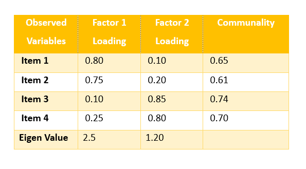
• • High loadings indicate strong relationships between observed variables and latent factors.
  • Item 1 and Item 2 load highly on Factor 1 (0.80, 0.75) – they likely represent one underlying concept.
  • Item 3 and Item 4 load highly on Factor 2 (0.85, 0.80) – they likely represent a different underlying concept.
  • Cross-loadings are low, indicating a clean factor structure.

Communality

• • Shows the proportion of each item’s variance explained by the factors.
  • Item 1: 65% variance explained.
  • Item 2: 61% variance explained.
  • Item 3: 74% variance explained.
  • Item 4: 70% variance explained.
  • High communalities (above 0.5) suggest the items fit well into the factor model.

Eigenvalues

• • Factor 1 eigenvalue (2.50): explains the variance equivalent to 2.5 observed variables.
  • Factor 2 eigenvalue (1.20): explains the variance equivalent to 1.2 observed variables.
  • Factors with eigenvalues >1 are generally considered significant (Kaiser’s criterion).
  • Factor 1 is the dominant factor explaining more variance than Factor 2.

Extraction Methods in Factor Analysis

Extraction methods determine the initial factors that best explain the variance and relationships among observed variables. Here, we discuss three primary methods: Principal Component Analysis (PCA), Principal Axis Factoring (PAF), and Maximum Likelihood (ML).

PCA and PAF Difference

1. Principal Component Analysis (PCA)

PCA aims to reduce a large set of correlated variables into a smaller number of uncorrelated components that capture most of the variance (Jolliffe & Cadima, 2016). Although PCA is technically a data reduction technique rather than a true factor analysis method, it is frequently used due to its simplicity.

Characteristics:

• • Focus: Captures total variance (common, unique, and error).
  • Components: Linear combinations of observed variables.
  • Assumptions: No distributional assumptions; does not separate unique and common variance.

Example: In a psychological test with 20 items, PCA might reduce the dataset to 3-4 components representing underlying abilities (e.g., verbal reasoning, memory).

Advantages:

• • Simplifies data and facilitates visualization.
  • Useful when the goal is dimensionality reduction.

Limitations:

• • Components may not represent true latent constructs.
  • Includes unique and error variance in its analysis.

2. Principal Axis Factoring (PAF)

PAF focuses on common variance shared among variables, excluding unique and error variance (De Winter & Dodou, 2012). It aims to uncover latent constructs that influence observed variables.

Characteristics:

• • Focus: Common variance only.
  • Assumptions: Moderate; initial communalities estimated iteratively.
  • Communalities: Initially estimated using squared multiple correlations and updated iteratively.

Example: In educational research, PAF could reveal underlying factors like motivation and test anxiety influencing student performance on a test.

Advantages:

• • Identifies latent constructs more accurately than PCA.
  • Better suited for theory development.

Limitations:

• • Iterative estimation may be computationally intensive.
  • Requires careful consideration of communalities.

3. Maximum Likelihood (ML) Factor Analysis

ML estimates factor loadings that maximize the likelihood of observing the sample data under a multivariate normal model. It provides statistical tests of model fit and parameter estimates with confidence intervals (De Winter & Dodou, 2012).

Characteristics:

• • Focus: Common variance.
  • Assumptions: Multivariate normality and linearity.
  • Statistical Testing: Enables tests for model goodness-of-fit and the number of factors.

Example: In validating a psychological scale, ML can test whether a hypothesized factor structure fits the data, allowing researchers to refine their model.

Advantages:

• • Provides formal tests of fit and confidence intervals.
  • Suitable for hypothesis-driven research.

Limitations:

• • Assumes multivariate normality, which may not always hold.
  • Computationally intensive for large datasets.

Rotation Methods in Factor Analysis

When we perform factor analysis, we are essentially trying to uncover patterns of relationships among observed variables (like test scores or survey items) that can be explained by a smaller number of underlying factors. Initially, factor analysis extracts these factors, but the resulting patterns—called factor loadings—are often complex and hard to interpret.

For example, without rotation, a variable might show moderate correlations with several factors, making it unclear which factor it really belongs to.

Orthogonal vs Oblique Rotation

There are two main types of rotation:

1. Orthogonal Rotation

Assumes that the factors are independent (i.e., uncorrelated). The “axes” representing the factors stay at right angles (90°) to each other. Makes the factor structure simpler by maximizing high loadings on one factor and minimizing loadings on others while keeping factors uncorrelated.

Subtypes of Orthogonal Rotation:

• • Varimax- Focuses on maximizing the variance of squared loadings for each factor. Produces factors with high loadings for a few variables and near-zero loadings for the rest. Commonly used because it provides a “clean” factor structure.
  • Quartimax- Simplifies the structure for each variable (row), pushing each variable to load strongly on one factor. Can result in one dominant “general factor” (e.g., overall ability or general health).
  • Equamax- A hybrid of Varimax and Quartimax. Tries to balance simplification of both variables and factors.

2. Oblique Rotation

Allows the factors to be correlated (i.e., factors can influence each other). The “axes” representing factors are not constrained to 90° angles. Reflects the reality that psychological and social constructs (like anxiety and depression) are often related, providing a more accurate and flexible solution.

Subtypes of Oblique Rotation:

• • Direct Oblimin- Allows for a range of factor correlations, controlled by a “delta” parameter (a setting chosen by the researcher). Suitable when some factors are expected to be weakly or moderately correlated.
  • Promax- Starts with an orthogonal (Varimax) rotation, then allows the factors to tilt and become correlated. Faster than Direct Oblimin, especially for large datasets.

Higher-Order Factor Analysis

Higher-order factor analysis involves applying a second-level factor analysis to the factor loadings obtained from an initial analysis. This technique is used when first-order factors are themselves correlated, suggesting the presence of overarching constructs.

Example: In intelligence research, specific abilities (e.g., verbal, spatial) may load onto a higher-order general intelligence factor (g).

Advantages:

• • Provides insights into the hierarchical structure of constructs.
  • Facilitates the development of complex theoretical models.

Challenges:

• • Requires large samples and careful model specification.
  • Interpretation can be complex.

Exploratory Factor Analysis (EFA)

EFA is used when researchers do not have a predefined hypothesis about the factor structure. It helps identify the number and nature of latent factors.

Steps in EFA:

1. 1. Data Adequacy: Test using KMO and Bartlett’s Test of Sphericity.
   2. Extraction: Choose an extraction method (e.g., PCA, PAF, ML).
   3. Determine Number of Factors: Use eigenvalues (>1), scree plot, or parallel analysis.
   4. Rotation: Apply orthogonal or oblique rotation.
   5. Interpretation: Analyze rotated loadings to understand factor structure.

EFA is widely used in scale development and theory exploration (Osborne & Costello, 2005).

Confirmatory Factor Analysis (CFA)

CFA tests specific hypotheses about the factor structure. Researchers specify the number of factors and which variables load on each factor.

Steps in CFA:

• • Model Specification: Define expected factor structure.
  • Model Estimation: Use software (e.g., AMOS, LISREL) to estimate parameters.
  • Model Evaluation: Use indices such as Chi-square, RMSEA, CFI, and TLI to assess fit.
  • Modification: Revise the model if necessary.

CFA is essential for validating measurement instruments and testing theoretical models (Kline, 2016).

Conclusion

Factor analysis is an indispensable tool for understanding the underlying structure of complex datasets. By employing methods like PCA, PAF, and ML, researchers can extract meaningful factors, rotate them for clearer interpretation, and use EFA or CFA depending on their research goals. Higher-order factor analysis adds another layer of sophistication, unveiling hierarchical structures that reflect real-world complexities. Mastery of these methods enables researchers to build robust theories and valid measurement instruments.

References

De Winter, J. C. F., & Dodou, D. (2012). Factor recovery by principal axis factoring and maximum likelihood factor analysis as a function of factor pattern and sample size. Journal of Applied Statistics, 39(4), 695–710. https://doi.org/10.1080/02664763.2011.610445

Fabrigar, L. R., Wegener, D. T., MacCallum, R. C., & Strahan, E. J. (1999). Evaluating the use of exploratory factor analysis in psychological research. Psychological Methods, 4(3), 272–299. https://doi.org/10.1037/1082-989X.4.3.272

Jolliffe, I. T., & Cadima, J. (2016). Principal component analysis: A review and recent developments. Philosophical Transactions of the Royal Society A: Mathematical, Physical and Engineering Sciences, 374(2065), 20150202. https://doi.org/10.1098/rsta.2015.0202

Kline, R. B. (2016). Principles and practice of structural equation modeling (4th ed.). Guilford Press.

Osborne, J. W., & Costello, A. B. (2005). Best practices in exploratory factor analysis: Four recommendations for getting the most from your analysis. Practical Assessment, Research & Evaluation, 10(7), 1–9. https://doi.org/10.7275/jyj1-4868